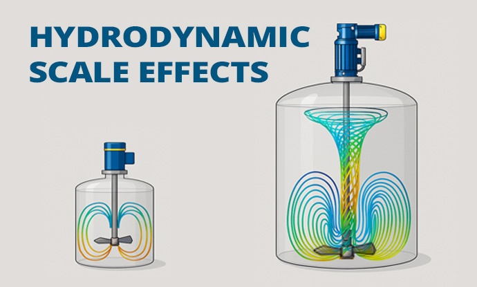
Understanding hydrodynamic scale effects when scaling up mixing systems

The agitation and mixing of fluids are essential operations in process engineering. A major challenge lies in scaling up a process from a small scale (laboratory or pilot) to a much larger industrial scale, whilst maintaining the same mixing performance. However, fluid flows do not simply ‘follow’ the geometric scaling: a change in scale profoundly alters hydrodynamic behaviour. This raises several scientific and technical issues: the influence of scale on the flow regime(laminar, transitional, turbulent), the consequences of the transition between these regimes on turbulence intensity and mixing quality, as well as the discrepancy between global phenomena (averaged over the vessel) and local phenomena(in certain regions of the fluid), for example in terms of velocity distribution and local concentration gradients. We address each of these aspects below, in order to explain why the change of scale in hydrodynamics is a complex issue, and how it can be overcome.

 

The effect of a change in scale on flow regimes

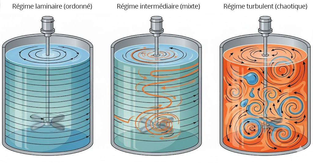
In agitated mixing, the flow behaviour depends heavily on the hydrodynamic regime. The following are typically distinguished:

• Laminar flow:

where the flow is orderly, consisting of layers sliding over one another without transverse fluctuations. Viscous forces largely dominate the fluid’s inertial forces. In practical terms, the fluid mainly follows the motion imposed by the stirrer without creating lateral eddies. There is no turbulence and mixing occurs solely through molecular diffusion, which is very inefficient. This regime generally prevails in highly viscous fluids or at very low stirring speeds.

• A turbulent regime:

where the flow is chaotic, with movements in all directions and across a wide range of scales. Inertial forces (linked to the fluid’s movements) outweigh viscous forces, so that the fluid’s viscosity has virtually no influence on macroscopic phenomena such as power consumption, flow rate or the size of the well-mixed zones. This regime is characterised by intense mixing: vortices form and dissipate continuously, ensuring rapid and homogeneous mixing of the fluid. In fully turbulent flow, the mixing of fluid streams is excellent.

• An intermediate (transient) regime:

between the two previous regimes, a mixed regime is observed where neither viscosity nor inertia completely dominates. In this zone, part of the flow exhibits fluctuations (partial turbulence), whilst another part remains orderly. According to standard criteria, this regime is observed for Reynolds numbers (a dimensionless number characterising the ratio between inertia and viscosity) ranging from approximately 10 to 10⁴. The threshold for turbulent flow is higher for an axial-flow impeller, as its design tends to delay the onset of turbulence. In practice, the laminar–turbulent transition depends on the geometry of the agitator and the vessel. For example, for a Rushton-type radial-blade impeller with counter-blades, it has been experimentally observed that the turbulent regime sets in above Re ≈ 10⁴, the laminar regime below Re ≈ 10, and the intermediate regime between these two values. It should be noted that certain configurations may remain laminar even beyond these values (for example, with ‘tangential’ impellers producing little transverse movement).

The transition from one scale to another is often accompanied by a change in flow regime, if the agitation conditions are not adjusted. Indeed, the Reynolds number of the agitator Re is proportional to N times d² (where N is the rotational speed and d is the diameter of the propeller or turbine).

If the scale is increased by multiplying all dimensions (tank size, propeller diameter, etc.) by a factor F, the volume of liquid increases as F³. To maintain the same flow regime, the rotational speed N should in principle be adjusted to keep Re constant.

However, several scenarios are possible:

• Same rotational speed as on a small scale:

N remains constant, whilst d increases (d₂ = F, d₁). In this case, the Reynolds number increases sharply (proportional to F²). Thus, a flow that was laminar or transitional on a small prototype may become fully turbulent at industrial scale, provided the fluid is not too viscous. This may seem positive (we finally obtain turbulence that is beneficial to mixing), but beware: the power required to drive this giant turbulent flow becomes disproportionate. In turbulent flow, the power P absorbed by the agitator increases very sharply with velocity and size (P is proportional to N³d⁵ for a given impeller). In our case, P is multiplied by F⁵. For a moderate extrapolation, for example from a 10 L laboratory vessel to a 10 m³ reactor (F = 10 in linear dimensions, and therefore a factor of 1000 in volume), the power absorbed per cubic metre (specific power) would be multiplied by 100. In other words, attempting to maintain the same mixing time whilst keeping the same stirring speed would require a power per unit volume that is a hundred times greater – often unrealistic in industrial terms. This is why it is rarely possible to ‘run at the same speed’ on a large scale.

 

• Reduced stirring speed:

In practice, to avoid excessive power requirements, it is often decided to reduce the rotational speed on a large scale. Taking the previous example (10 L ➜ 10 m³), reducing the rotational speed by a factor of approximately 4 would be sufficient to avoid this surge in power: the specific power would only increase by ~60% (instead of 100×). However, this reduction in speed comes at a cost: it increases the mixing time. In this case, by dividing N by 4, one should expect the time required to homogenise the tank to be approximately four times longer than in the laboratory. Furthermore, lower velocity implies a lower Reynolds number: the risk is then of deteriorating the flow regime, possibly reverting to the transitional or even laminar regime if the fluid is viscous. This is a typical trade-off associated with scaling up: it involves accepting slower mixing to remain within manageable power and velocity ranges. Another approach involves modifying certain geometric parameters during the scale-up. For example, a larger impeller relative to the tank can be used at industrial scale than in the laboratory (increasing the d/D ratio of the impeller diameter to the tank diameter) to promote more vigorous mixing without excessively increasing the rotational speed. Similarly, it is possible to add several agitator stages on the same shaft in a very tall vessel, in order to mix all the upper zones. These ‘non-geometric’ adaptations sometimes allow several similarity criteria to be maintained simultaneously (for example, a certain turbulence intensity whilst keeping power consumption in check). On the other hand, they complicate the design and direct comparison with the laboratory scale.
 

• Design adjustments:

In summary, the effect of scale on the flow regime can be summarised as follows: without precautions, a change of scale can cause a flow to switch from one regime to another. Moving from a laminar regime (poorly mixed) to a turbulentregime (well mixed) may seem beneficial, but it comes with significantly higher energy requirements. Conversely, if power is limited at large scale, there is a risk of falling into a less efficient transitional regime. Ideally, the agitator engineer aims to operate in a turbulent regime as much as possible, as this ensures rapid and homogeneous mixing. However, achieving this regime in a large volume often requires either investing in agitation power or developing solutions (geometry, multiple agitators) to promote turbulence despite the scale. It is therefore easy to see that extrapolating from a stirred tank is no simple matter: it is necessary to determine which parameters to keep constant and which may vary, so as to reproduce the process on a large scale without any loss of performance. We will return later to the similarity criteria used for this purpose.

Transition between regimes: consequences for turbulence and mixing quality

It is generally advisable to avoid operating a mixer in the transitional regime. Indeed, the laminar–turbulent transition is accompanied by a significant variation in flow characteristics, which can adversely affect mixing quality. Several problems may arise in the transitional regime:
 

• Incomplete turbulence

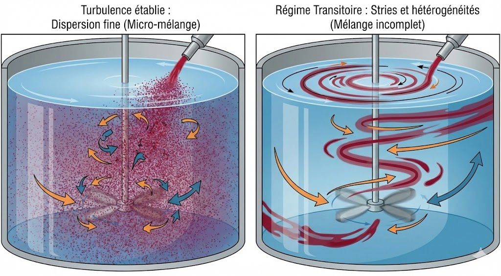
When fully established, turbulence manifests itself as rapid fluctuations in velocity at all scales, which greatly improves mixing at fine scales (this is referred to as micro-mixing). In the intermediate regime, turbulence is only partial. The fluid is not entirely calm, but neither is it completely chaotic. Vortices may appear and then disappear, in an irregular manner. This sporadic turbulence means that the mixing only partially benefits from the advantages of the turbulent regime. Turbulent intensity (measured by the amplitude of velocity fluctuations) is lower and less uniform than in a fully turbulent regime. Consequently, the fragmentation of unmixed zones is less pronounced: there remain areas where the fluids do not disperse well. In other words, the quality of the mixing is reduced compared to pure turbulent flow. For example, a stirred tank in transient flow may exhibit streaks or pockets of less well-mixed liquid, whereas turbulent stirring would homogenise the entire contents.

• Sensitivity and unpredictability:

The intermediate regime is often unstable and sensitive to disturbances. Small changes in stirring speed, fluid viscosity or geometry can cause it to oscillate towards a more laminar or more turbulent state. This unpredictability complicates mixing control and scale-up: empirical correlations (for example, for mixing time, mass transfer coefficient, etc.) are less reliable in this regime. In purely laminar or purely turbulent flow, models are established – for example, the power dissipation P varies linearly with N in laminar flow (Stokes’ law) and with N³ in turbulent flow (power law). But in the intermediate regime, the relationship P(N) or other quantities evolve in a complex non-linear manner, making extrapolations uncertain.

• Poor macroscopic mixing:

If the intermediate regime persists on a large scale, the risk is that we accumulate the disadvantages of both regimes without reaping all their benefits. On the one hand, the flow is not turbulent enough to stir the volume thoroughly and quickly, so overall mixing takes longer. On the other hand, the flow is sufficiently chaotic to prevent reliance on regular laminar circulation to distribute the fluids uniformly. This can result in heterogeneous mixing, with some areas well-mixed and others almost stagnant. For example, during a liquid-liquid mixing process in a transitional regime, large ‘fingers’ of one liquid may form within the other, which take a long time to dissipate. Similarly, when dissolving a solid, the transitional regime may not provide sufficient shear to break up the aggregates, whilst dispersing them into random areas of the vessel.

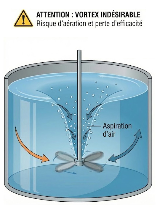
• Vortex risks:

A specific case related to the transition involves the formation of vortices at the free surface. 

In turbulent flow with anti-vortex vanes (anti-vortex deflectors), the surface remains relatively flat because the vortex movements are quickly disrupted by the turbulence and the vanes.
 

In laminar flow, the surface also remains flat because the fluid rotates as a single unit without forming a central depression. However, under certain intermediate conditions (particularly without baffles or with moderate agitation), a vortex may form. This vortex is undesirable because it can draw air into the tank (which disrupts the mixing and causes foaming or oxidation) and because it indicates inefficient use of energy (some of the energy is used to maintain this vortex rather than for mixing).
 

The formation of a vortex is associated with a high Froude number, i.e. a regime dominated by centrifugal inertia relative to gravity. With effective counter-blades, this problem is generally eliminated, but at too low a velocity (or without sufficient turbulence), the liquid may remain in quasi-rigid rotation and form a stable vortex. This phenomenon typically occurs at a moderate Reynolds number (it is observed from Re approx. 300 in an unobstructed tank), i.e. in a transitional regime in many cases. The solution is either to increase turbulence (by increasing N or modifying the geometry) to break up the vortex, or to add/repair the baffles.

In short, the best mixing is achieved under fully developed turbulent flow.

Any transitional state in which this optimal flow regime is not achieved results in slower, or even less homogeneous, mixing. This is why, when scaling up a process, the process engineer seeks to ensure that the large-scale system operates under the most favourable flow conditions possible. For example, in the case of a highly viscous fluid (polymers, syrups, etc.), it is sometimes unavoidable to remain in laminar flow at industrial scale; the agitator will then be sized to at least achieve effective laminar flow (using an impeller such as an anchor or ribbon propeller, which covers the wall effectively, to eliminate stagnant zones). Conversely, for a low-viscosity fluid, it is important to ensure that the agitation system provides sufficient energy to clearly exceed the transition and enter a turbulent regime, using a similarity criterion such as the constant power number (which guarantees a certain level of turbulence at every scale). Finally, the intermediate zone should be avoided during gradual scale-ups: in practice, it is recommended to proceed in size steps (from lab to pilot, then to demonstrator, then to industrial scale) with reasonable increments (for example, a factor of 10 in volume each time), so as to be able to adjust the conditions and avoid sudden hydrodynamic variations that could otherwise degrade performance.

Local phenomena vs global phenomena: velocity heterogeneity and gradients

Another challenge related to the scale effect is taking into account local phenomena within the fluid, as opposed to global measurements. At the laboratory scale, global parameters are often the primary focus: for example, mixing time (the time required to homogenise the entire tank), total agitation power, average circulation flow rate, etc. However, in a large industrial tank, the flow is far from uniform: it exhibits a highly heterogeneous 3D structure, particularly in turbulent flow. There are profiles of velocity, shear, turbulence intensity, concentration, temperature, etc., varying from one point to another within the tank. Local analysis of the flow, via measurements (anemometry, PIV laser velocimetry) or CFD simulations, reveals, for example, the existence of dead zones (with little or no mixing, often in corners, at the top or near the walls) and high-shear zones (generally in the immediate vicinity of the moving object). In other words, at any given moment, different regions of the reactor are subject to very different hydrodynamic conditions.

Thus, the fluid elements or dispersed inclusions (solid particles, liquid droplets, gas bubbles, microorganisms, etc.) present in the tank do not all experience the same local environment. For example, a microbe circulating near the impeller will be subjected to high velocities and high shear (which can improve nutrient transfer but also risks damaging fragile cells), whilst another microbe located in a remote corner may lack dissolved oxygen or substrate due to the lack of rapid liquid renewal.

Similarly, in a chemical reactor, concentration or temperature gradients may persist locally: if a reactive species diffuses poorly within the vessel, concentration heterogeneities may affect reaction kinetics or lead to undesirable by-products. Thus, on a large scale, process performance may also depend on these local phenomena. A mixture that is broadly “homogeneous” may conceal micro-heterogeneities which, if they coincide with the characteristic scales of the process (reaction, cell growth, etc.), will have negative impacts on yield or product quality.

To control these effects, it is essential to supplement the global study with a local study of the stirred tank. In practical terms, this means focusing on the three-dimensional distribution of velocities and gradients, and seeking to make it compatible with the process requirements. Let us compare, for example, the size of turbulent vortices with the dimensions of the particles or microorganisms: if the vortices are much larger, the particles essentially ‘experience’ an average flow without being finely dispersed; if they are smaller, on the other hand, they agitate each particle effectively. It is also possible to evaluate the residence time of a fluid at a given point (related to the flow rate) in relation to the characteristic reaction time: if mixing is too slow locally, the reaction will take place in a non-equilibrium state, potentially resulting in incomplete conversion or localised hot spots.

A useful concept is that mixing actually occurs via several complementary mechanisms:

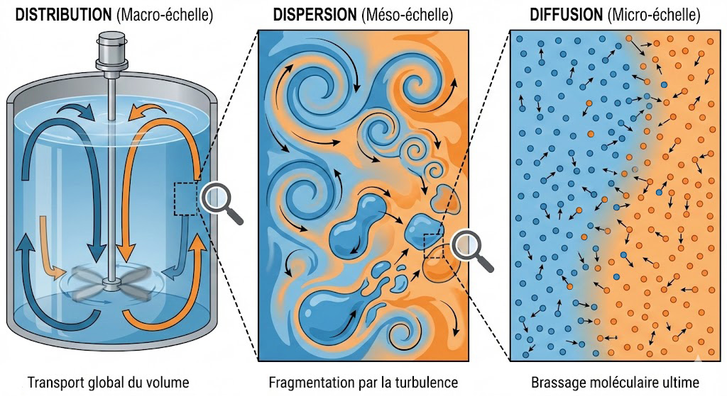
• Distribution (or overall convection): the transport of the fluid by the main currents generated by the stirrer, so as to sweep through the entire volume. This process helps to bring different regions of the fluid into contact, but it becomes slower the larger the volume to be covered. Indeed, a larger volume means longer circulation distances and an increased risk of areas that are difficult to reach. On a small scale, distribution is relatively rapid (it is easy to mix an entire 1-litre beaker using a magnetic stirrer). On the scale of a 50 m³ tank, however, even a strong current will take some time to carry fluid from one end to the other: this principle is commonly referred to as ‘volume inertia’.

• Diffusion: mixing at the molecular scale via Brownian motion, causing molecules to move from more concentrated areas to more diluted areas. This is the ultimate phenomenon that homogenises the fluid at the microscopic level (beyond what dispersion has been able to achieve). Pure diffusion is very slow on the scale of a tank (for example, allowing sugar to diffuse without stirring would take hours in a glass of water), but very rapid over short distances. This is why prior dispersion is crucial: the more successfully agitation has reduced the size of the fluid pockets to be mixed, the more quickly diffusion can finish the job. In other words, turbulence creates small, well-mixed elements, and diffusion takes care of eliminating the final concentration gradients between these elements.

• Dispersion: the fragmentation of fluid elements by the action of turbulence through a shearing effect, forming a multitude of fluid particles of increasingly smaller size and homogeneous composition, which disperse throughout the entire volume. Dispersion is essentially due to vortices: large vortices mix large volumes together, whilst, as they break up into smaller vortices, they also mix volumes on a smaller scale. In intense turbulent flow, dispersion produces an intimate mixing of the fluids, down to very fine scales. In laminar flow, by contrast, there is no dispersion due to turbulence; different fluid layers can coexist for a long time without subdividing, which delays complete mixing.

These three mechanisms act in concert in a real mixture. On a small scale, the mixing engineer often manages to implement all of them effectively: a laboratory mixer creates both good circulation (distribution) and sufficient turbulence (dispersion), so that diffusion need only balance out a few final traces of gradient. On a large scale, however, the weak link may be distribution: it is possible to generate a great deal of turbulence locally, but if certain areas of the vessel are not adequately supplied with agitated fluid, they will remain poorly mixed.
 

For example, a large, high-speed agitator can create a highly turbulent jet in its immediate vicinity, but if this jet does not penetrate to the bottom of the vessel, the bottom may remain stratified. This is where judicious design choices come into play: the geometry of the tank and the agitator; the position, type and number of blades; the presence of counter-blades, etc. play a crucial role in ensuring uniform mixing. Anti-vortex devices (counter-blades) are almost always essential in cylindrical tanks to break up purely tangential circular motion and induce useful radial and axial flows. Without these deflectors, the liquid could simply rotate as a mass without ever actually mixing transversely (stable or centrifugal vortex phenomenon).

Similarly, a slow-rotating impeller with a large diameter tends to move a large volume of fluid gently (significant axial flow), reaching the corners of the tank, whereas a small, fast-rotating impeller would merely shear the fluid locally without entraining the rest (concentrated radial flow). This is why, for large volumes, it is often recommended to use large-scale axial flow impellers, such as propellers or turbines set at an angle covering between one-third and two-thirds of the tank’s diameter (the ratio depending on the liquid’s viscosity), rather than a small, centrally positioned turbine. These “gentle” agitators ensure better overall distribution (fewer dead zones) whilst generating sufficient turbulence to disperse the fluids effectively.

Ultimately, local heterogeneity is a major scaling issue. For the same volume, a small vessel will tend to be more uniform than a large one, simply because every portion of fluid is closer to the agitator and travels shorter distances to mix. On a large scale, it is particularly difficult to prevent local velocity or concentration gradients from occurring; the aim is to minimise them and ensure they do not compromise the process. Recent advances in computational fluid dynamics (CFD) and metrology have enabled a better characterisation of these local phenomena. It is now possible to visualise velocity or turbulent energy maps within the tank. This information is invaluable for identifying, for example, a dead zone beneath a radial impeller (which could be corrected by lowering the impeller or adding a second stage), or a region of intense, potentially damaging shear (which could be mitigated by selecting a less aggressive agitator). In summary, a detailed understanding of the velocity distribution and local gradients on a large scale enables the optimisation of the design and operation of industrial mixers, in order to meet the challenge of achieving mixing that is as homogeneous and controlled as in the laboratory.

Conclusion

Scaling up in hydrodynamics represents a multidimensional challenge. On the one hand, it involves ensuring an appropriate flow regime is maintained whilst balancing similarity criteria: keeping the Reynolds number sufficiently high to benefit from turbulence, without requiring unrealistic power. On the other hand, it is important to take into account local mixing constraints: a large tank requires circulation that covers the entire volume and ensures that every corner receives sufficient mixing energy, in order to avoid poorly mixed pockets and harmful gradients.

In practice, the scaling strategy often involves selecting one or two key parameters to retain between the pilot and industrial scales, depending on the process objectives. Often, several iterations are required: upscaling, identifying discrepancies (through simulation or pilot tests), then adjustment (for example, by modifying the impeller diameter, adding counter-blades or changing the similarity rule). Proceeding in stages allows these adjustments to be refined progressively.

In doing so, hydrodynamic scaling effects necessitate a re-evaluation of the mixing process with every change in scale. However, thanks to advances in fluid science, it is possible to anticipate these challenges and overcome them: today, agitator designers know how to combine global analysis (power balance, mixing time) and local analysis (velocity profiles, turbulence scales) to design robust agitation systems tailored to the volume to be processed.